Tutorial
For a tutorial on the free demonstration version of Ranges, see the Demo Tutorial.
Introduction
This is a brief tutorial to work you through the basics of using Ranges. It concentrates on the practical steps you need to take to perform different analyses. It contains little explanation of what the routines do (see overview and links from there for that).
Lines starting with a bullet point (•) describe actions to perform. Click on the images to the right to enlarge them.
Getting your data in and viewing
Location data, the simplest option - just coordinates for a single range
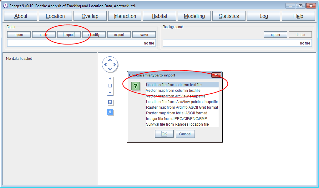
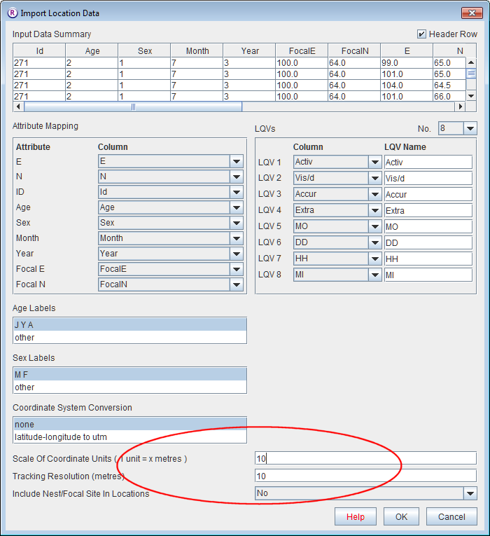
- Open Ranges to the main window
- Press import and select Location column file
- Select the file <RangesFolder>\samples\blackbird\blackbird_indiv1_coords_only.txt
If you look at this file in a spreadsheet you’ll see it contains 2 columns of data with the headers E & N.
The import routine detects the file contents, and sets up the defaults accordingly.
- Set Scale Of Coordinate Units and Tracking resolution to 10. Press OK to accept other defaults
This will have read the two columns in as a single range, the points will be displayed in the map display and you can alter range attributes in the Ranges table, or the coordinates themselves in the Location table.
- Press save to save this as a Ranges location file that can be used as an input in other Ranges routines.
(Note that an alternative way of doing this is to press new, then open the text file in Excel, copy the coordinates and paste them into the empty locations table).
Location data - coordinates for multiple ranges
- Open Ranges to the main window
- Press import and select Location file from column text file
- Select the file <RangesFolder>\samples\blackbird\blackbird_ids_and_coords.txt
If you look at this file in a spreadsheet you’ll see it contains 3 columns of data with the headers ID, E & N.
- Set Scale Of Coordinate Units and Tracking Resolution to 10. Press OK to accept the defaults.
This will have read the coordinates into four ranges according to the ID specified in the first column.
- Press save to save this as a Ranges location file.
Location data - coordinates, range attributes and location qualifying variables
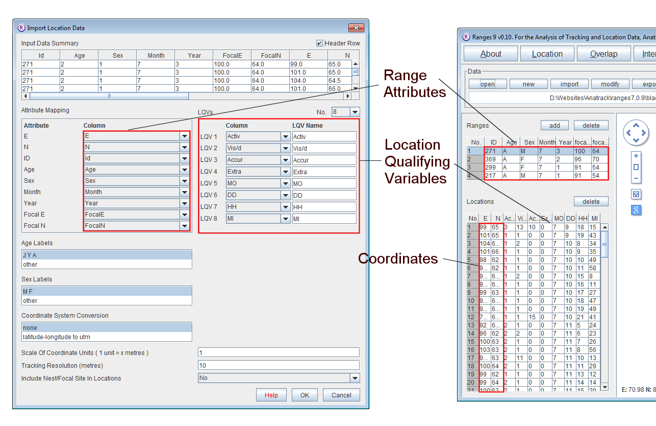
- Open Ranges to the main window
- Press import and select Location file from column textfile.
- Select the file <RangesFolder>\samples\blackbird\blackbird.txt
If you look at this file in a spreadsheet you’ll see it contains 17 columns of data.
- Set Scale Of Coordinate Units and Tracking Resolution to 10. Press OK to accept the defaults.
This will have read the coordinates into four ranges as above, but it will also have read in range attribute data that will be displayed in the Ranges table and location qualifying variables that will be displayed in the Locations table.
- Press save to save this as a Ranges location file, but note that an identical file named blackbird.loc is already provided in the blackbird directory.
Viewing a large multi-range file
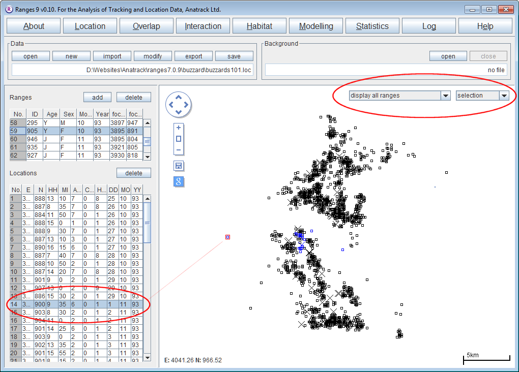
- Open Ranges to the main window
- Press open and select <RangesFolder>\samples\buzzard\buzzards101.loc
- Above the map display, change from display selected range(s) to display all ranges
- Make sure the range colours next to the display option box is set to selection
- Click the left mouse button in the left column of the Ranges table.
- Use the arrow keys to move down the table (see how the selected range is displayed in blue, and the data for the selected range is displayed in the Locations table.
- Select the left column in the Locations table.
- Use the arrow keys to move between locations in the table.
See how the selected location is circled in red.
- Left click on a blue location in the map display while holding down the SHIFT key.
See how the corresponding row in the Locations table becomes selected, and the location is coloured red to show that it is selected.
- Try editing the E or N values for a location in the Locations table and see how its position in the map display is changed.
- Change the range colour option box to ‘sex’.
You will see males displayed in blue and females in red.
Viewing GPS collected movement paths with associated time information
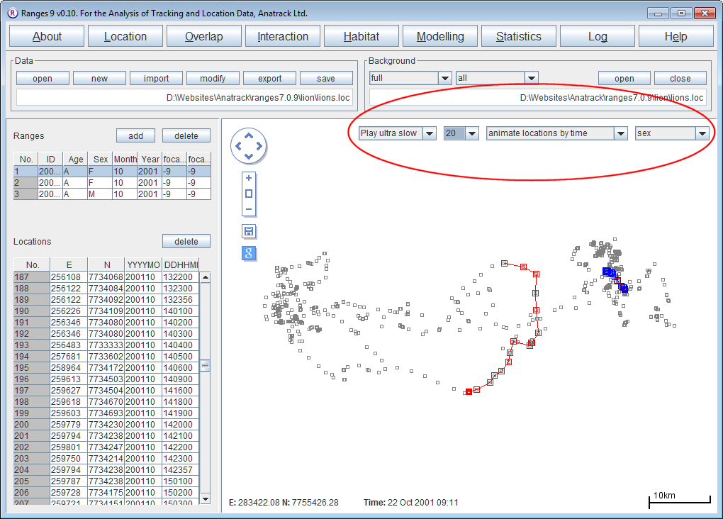
- Open Ranges to the main window
- Press open and select <RangesFolder>\samples\lion\lions.loc
- Above the map display change from display selected range(s) to display all ranges
- Change the range colour to sex.
You should see the male locations overlapping with those of the two females.
- Tick Background map and browse to select lions.loc as the background file too.
- Above the map display, change from display all ranges to animate locations by time.
- Change the option from Play fast to Play med or slower
You should be able to follow the movements of the 3 individuals over time, the first female enters the area covered by the male on the 20th of October and leaves on the 21st, the male doesn’t enter the area covered by the first female until the 27th.
Location analyses
Inter-location distances
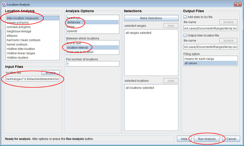
- Click on the Location button to open the Location Analysis setup window.
- Choose inter-location measures.
- Under Input Files press browse and find the file <RangesFolder>\samples\blackbird\blackbird.loc.
- Under Analysis Options, select distances, location interval and leave the Per number of locations set at 1.
- Press the Run Analysis button.
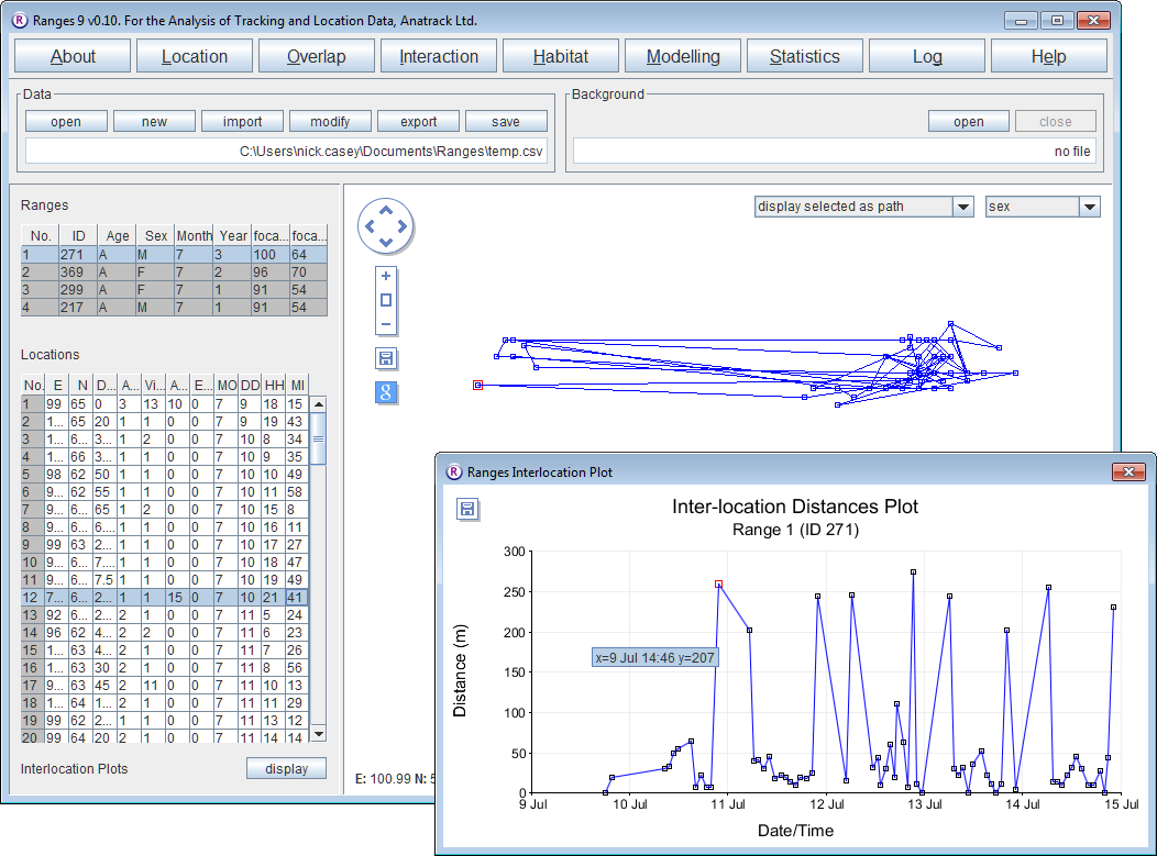
The progress window will flash up (this is a fast-running analysis. Then the Statistics window and a Plot window will be displayed over the main window.
- Select different ranges within the ranges table on the upper left.
The results for them will be displayed in the Plot window.
- Select different locations in the locations table on the lower left and the corresponding location will be displayed in red in the plot.
Note that a new column Distances(m) has been added to the file in the Locations table.
100% Minimum convex polygons
- Click on the Location button to open the Location Analysis setup window.
- Choose convex polygons
- If a file is not loaded, under Input Files press browse and find the file <RangesFolder>\samples\blackbird\blackbird.loc.
- Under Analysis Options select 100% cores.
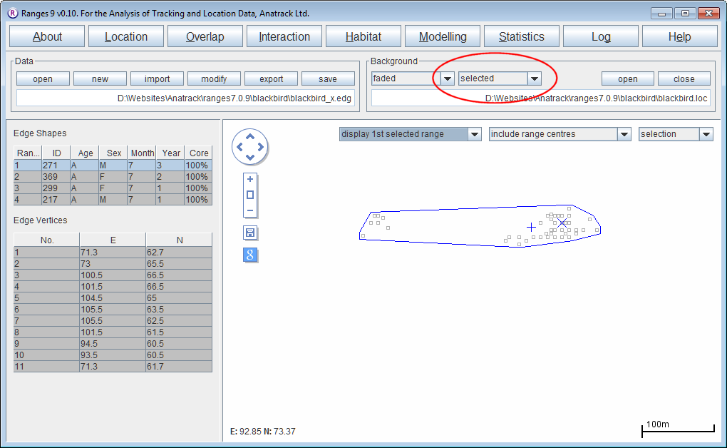
- In Output Files, select Output edge file and accept the default filename (blackbird_x.edg).
- Press the Run Analysis button.
The edge file created will be displayed in main window.
- Select different ranges in the Edge shapes table at the upper left.
The range edge and the locations used to create it will be displayed ( the latter occurs because the tickbox for selected is the current option for the Background.
If you wish to export the polygon edge file to ArcView or another GIS package do the following :
- From the main window press export, and select ArcView Shapefile Polyline.
Convex polygons at 5% intervals
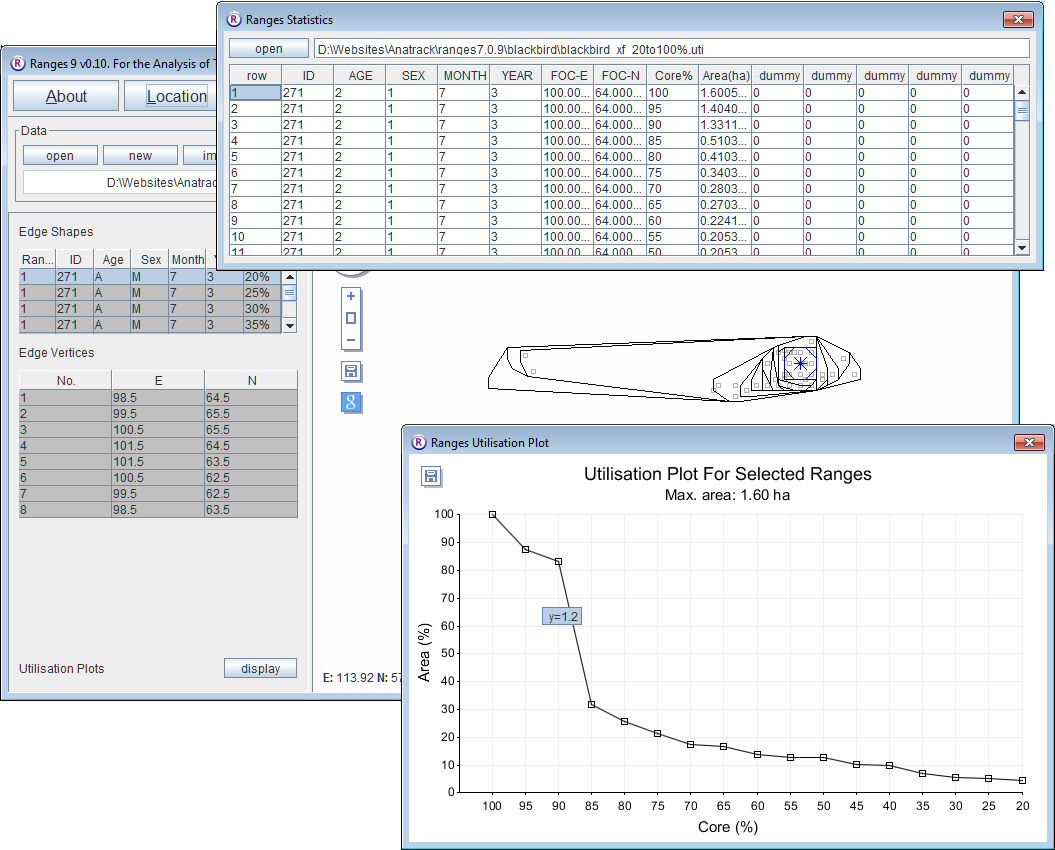
- Click on the Location button to open the Location Analysis setup window.
- Choose convex polygons.
- If a file is not loaded, under Input Files press browse and find the file <RangesFolder>\samples\blackbird\blackbird.loc.
- Under 'Analysis Options select cores at 5% intervals
- Under Peel centre select focal site (this means that locations will be excluded based upon their distance from the focal site).
- Press the Run Analysis button.
The cores, and a utilisation plot will be displayed in the main window for the first range.
- Select the first row in the upper left table and use the arrow key to move down through the range cores and on to the next ranges.
Incremental area plots
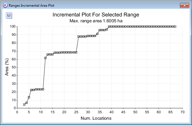
Incremental area plots display how the area of an estimated home range core changes as successive locations are added.
- repeat the steps in Convex polygons at 5% intervals, but before pressing Run Analysis change the following options :
- Under Analysis Options select incremental area analysis
- Keep the core % at the default value of 100.
- Press the Run Analysis button.
The incremental area plot will be displayed for each range in the main window.
Cluster analysis with objective cores
- Click on the Location button to open the Location Analysis setup window.
- Choose "neighbour-linkage.
- If a file is not loaded, under Input Files press browse and find the file <RangesFolder>\samples\squirrel\furzey.loc.
- Under 'Analysis Options select objective cores
- Under Linkage method select cluster convex polygons
- Leave Inclusive or cluster at the default of separate cluster polygons
- Leave Polygon display method at the default of corner & cell polygons; these options give the classic cluster analysis from Kenward (1987), Kenward et al. (2001)).
- Under Outlier exclusion select iterative alpha 0.1% (this choice gives the most conservative exclusive of outlying locations – i.e. the outlier exclusion distances are large) and hence only the most extremely excursive locations are excluded.
- Under Output files click the box to select output edge; this should create a file furzey_cxoi01s.edg
- Press the Run Analysis button.
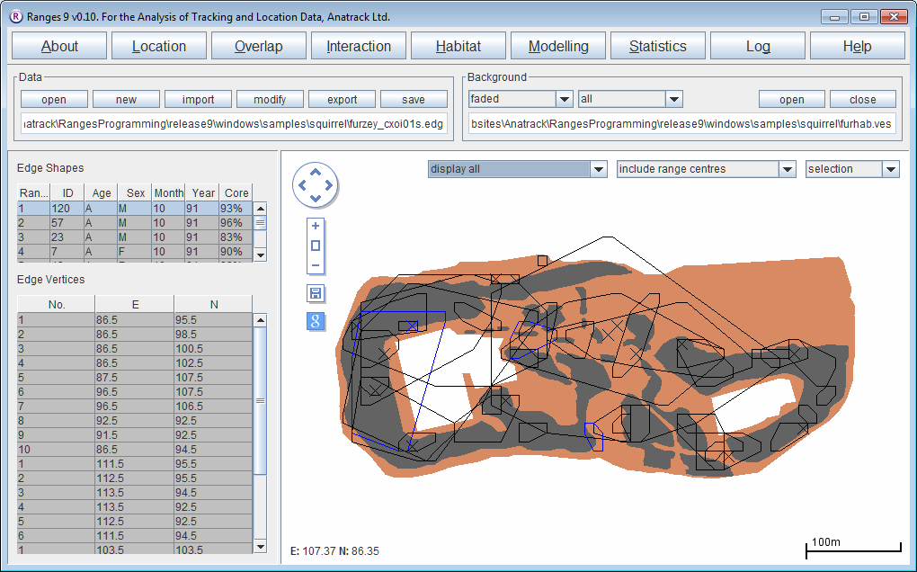
The edges will be displayed in the main window for the first range, with cluster analysis statistics see nuclei, partial area, diversity of areas and diversity of locations in the Glossary in a separate window.
- In the Outlier exclusion box at the top of the graphics screen, select display all.
- In the Background box above the graphics screen, press the (third) open button and select the file furhab.ves; in the same box select all instead of clipped in the second box.
The map of Furzey Island will plot in brown under the range outlines, with the (Scots pine) woodland used by the red squirrels shown in black. The island is surrounded by sea, and has two areas large of concrete used for oil-drilling within the woodland. Note that one squirrel location was on the beach to the north of the island, and (if you open the file furzey.loc instead of the edges in the Data box and select the (first) button to display the map faint in the Background box) that squirrels rarely used the oil-extraction sites.
Dispersal detection via inter-location distances
- Click on the Location button to open the Location Analysis setup window.
- Choose inter-location measures
- Under Input files press browse and find the file <RangesFolder>\samples\buzzard\buzzard_dispersal.loc.
- Under Analysis Options, select distances, site to location
- Tick the dispersal detection box
- Set Minimum dispersal distance’ to 1000 and Alpha for dispersal detection to none.
- Press the Run Analysis button.
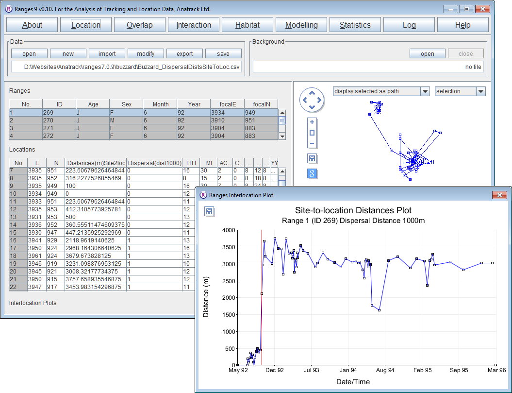
The distances from the focal site to each location over time for the first range will be displayed in a separate window, with a red vertical line marking where dispersal was classed to occur by the entered criteria.
- Select different ranges within the ranges table on the upper left and the results for them will be displayed in the plot window.
Note that new columns Distances* and Dispersal* have been added to the file in the Locations table. The latter contains 0 prior to dispersal and 1 after it.
Overlap analysis
Creating an overlap matrix
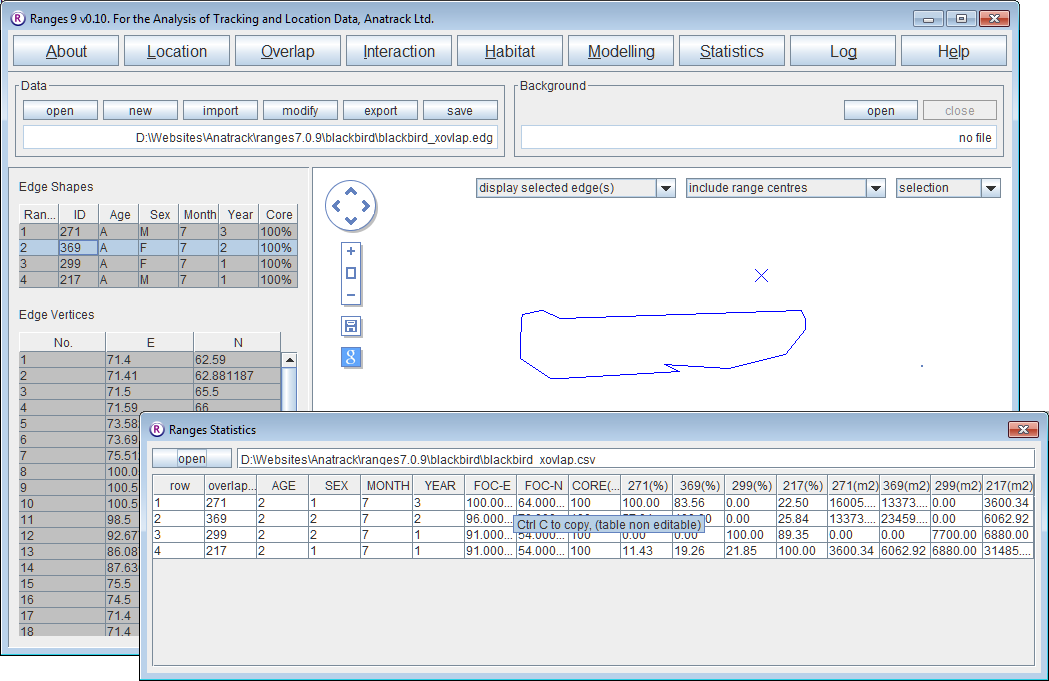
- If you have not already done so, run through 100% Minimum convex polygons to create the file blackbird_x.edg]].
- Click on the Overlap button.
- Select range overlap.
- Press browse and select the edge file <RangesFolder>\samples\blackbird\blackbird_x.edg
- Press the Run Analysis button.
In the statistics window and you will be able to see the percentage overlap of the ranges in rows by the ranges in columns followed by the area itself. A new map has been built of the union of each range's overlap with all the others.
Interaction analysis
Autocorrelations
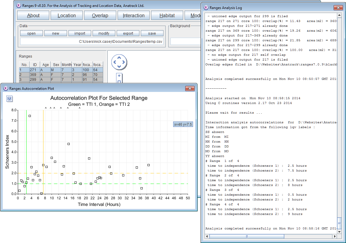
- Click on the Interaction button.
- Select autocorrelations.
- Press browse and select <RangesFolder>\samples\buzzard\buzzards.loc.
- Press the Run Analysis button.
- When the analysis has finished, click the Log button to see the time to independence (Schoeners 1) for each range. These are displayed in the plot.
Dynamic interactions

- Click on the Interaction button.
- Select dynamic interactions.
- Press browse and select <RangesFolder>\samples\lion\lions.loc.
- Select all'’ for Individual selection
- Select time attributes of locations for Same time observations defined by.
- Enter 30 for Input threshold between same-time observations (minutes).
Locations were collected approximately hourly; this will allow for the slight variation while not considering consecutive locations as being taken at the same time.
- Leave the default Maximum randomisation sample (5000).
- In Output files select 'means for each range.
- Press the Run Analysis button.
On completion, you should see in the statistics file that the Jacobs indices in the final three columns are less than 0.1 for all combinations except for the last one (which is for the second female and the male). This generates Jacobs indices of > 0.75 using the different means, indicating strong positive association between the movements.
Habitat analysis
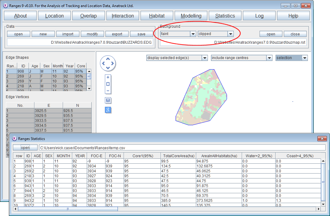
Habitat content of ranges
- Click on the Habitat button.
- Select habitat content of ranges.
- For the map file, press browse and select <RangesFolder>\samples\buzzard\buzzmap.rst.
- for the edge file, press browse and select <RangesFolder>\samples\buzzard\buzzards.edg.
- Press the Run Analysis button.
When the analysis completes, the statistics window will contain the area calculations for each habitat in each range.
The map in the main window contains the edge file in the foreground with the habitat raster in the background clipped to the edges and faint to make the edge lines clearer.
- To use a vector habitat file rather than a raster file use the files <RangesFolder>\samples\blackbird\blackbird_map.ves and <RangesFolder>\samples\blackbird\blackbird_x.edg (the latter created in 100% Minimum convex polygons).
Habitat in buffers around locations
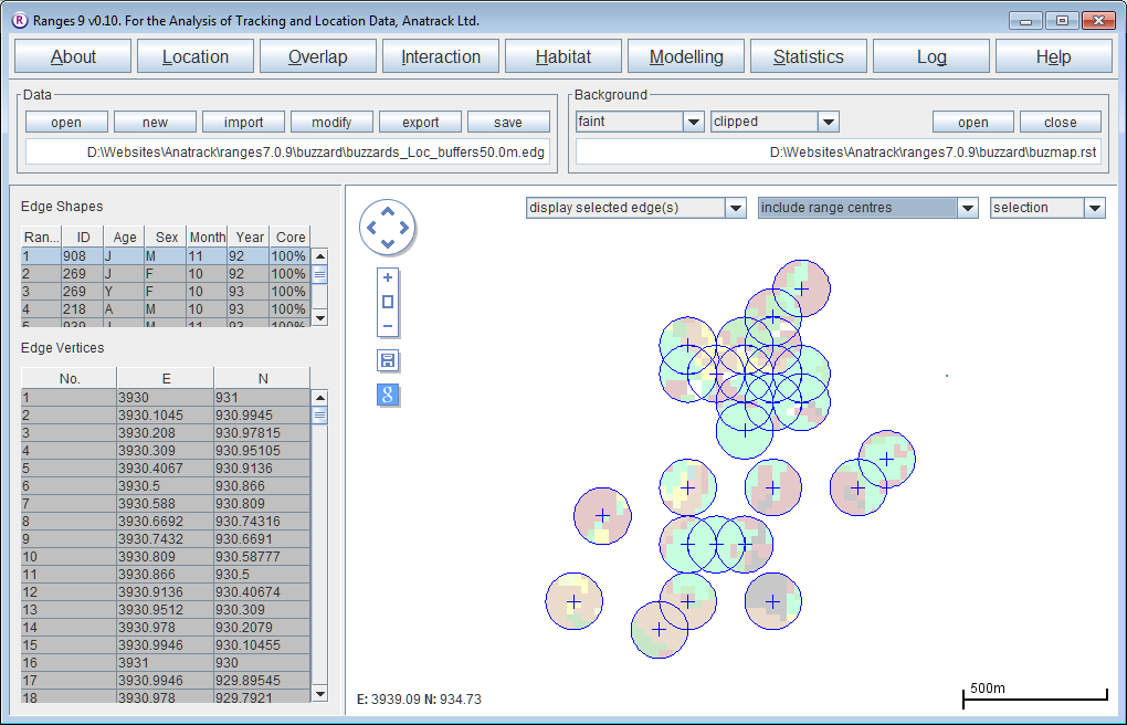
- Click on the Habitat button.
- Select habitat at locations.
- The map file should be already set but if not, press browse and select <RangesFolder>\samples\buzzard\buzzmap.rst.
- For the location file, press browse and select <RangesFolder>\samples\buzzard\buzzards.loc.
- In Analysis Options, select buffers around locations
- Change Input circle radius to 100.
- Press the Run Analysis button.
- When the analysis has finished, circles around each habitat will be displayed on the map.
Fish analyses, midline and clipping
Midline inter-location distances

- Click on the Location button to open the Location Analysis setup window.
- Choose midline inter-location.
- Under Input Files for location file, press browse and find the file <RangesFolder>\samples\fish\fish.loc.
- For the midline file, press browse and find the file <RangesFolder>\samples\fish\midline.vel.
- Under Analysis Options, select distances, location interval and leave the Per number of locations set at 1.
- Click the link midline to locations checkbox.
- Press the Run Analysis button.
The statistics file will contain the distances file. The main window map will display the paths between all locations on the map. To view each path individually:
- change from ‘display all’ to ‘display selected edge(s)’, and use the mouse or cursor keys to select different paths within the upper left table.
Midline linear ranges
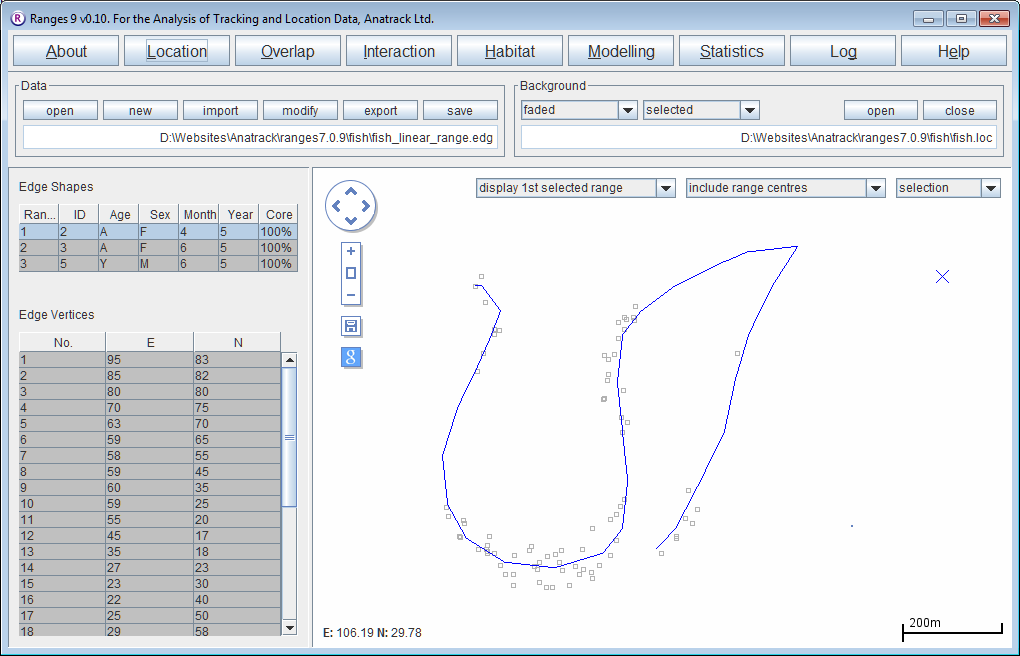
Using the same input files as above
- Select midline linear ranges
- Press the Run Analysis button.
The length of each linear range will be displayed in the statistics file. The main window map will display each linear range, with the locations in the background.
- Try changing the background map to <RangesFolder>\samples\fish\midline.vel to see how far the river extends beyond the fishes' range.
Clipping home ranges by a river outline
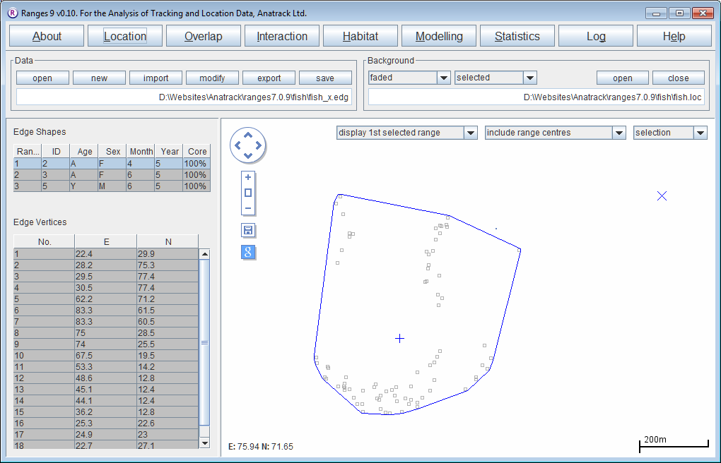
- Click on the Location button to open the Location Analysis setup window.
- Choose convex polygons, 100% cores
- Use the same location file as above (<RangesFolder>\samples\fish\fish.loc.)
- Check Output edge file in Output Files to create file <RangesFolder>\samples\fish\fish_x.edg.
- Press the Run Analysis button.
When the analysis is complete the map will show the convex polygon, with the locations in the background.
- Click on the Habitat button to open the Habitat Analysis setup window.
- Select ‘habitat content of ranges’
- For the map file, press browse and select <RangesFolder>\samples\fish\river.ves.
- For the edge file, press browse & select <RangesFolder>\samples\fish\fish_x.edg (created at the start of this exercise)
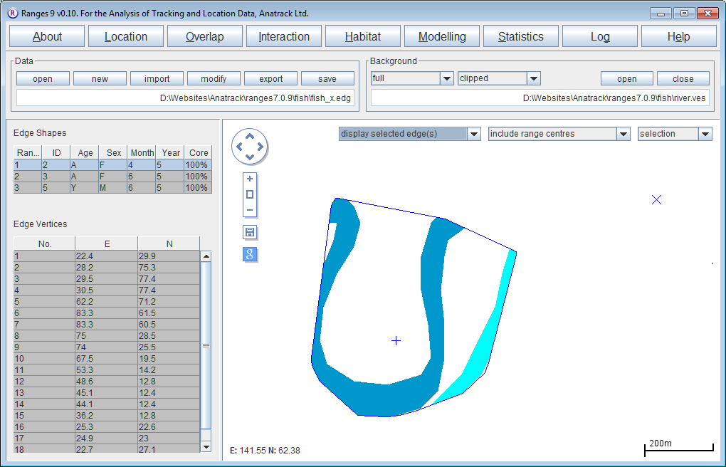
- Check Output clip file in Output Files to create file <RangesFolder>\samples\fish\fish_x_Hab_river_clip.edg.
- Press the Run Analysis button.
The clip file be loaded in the main window. You can load the original file fish_x.edg as a background to see the difference between them. The statistics will show the total area of the MCP, then the percentage of that area that is in the main river (dark blue) and tributary (light blue).
Modelling
These routines estimate resource-requirement and survival parameters which can be used in modelling. Future work will focus on refining these parameters and providing new ones with further automated analyses of the type being conducted in Resource Area Dependence Analysis.
Resource Area Dependence Analysis
Plotting observed data only
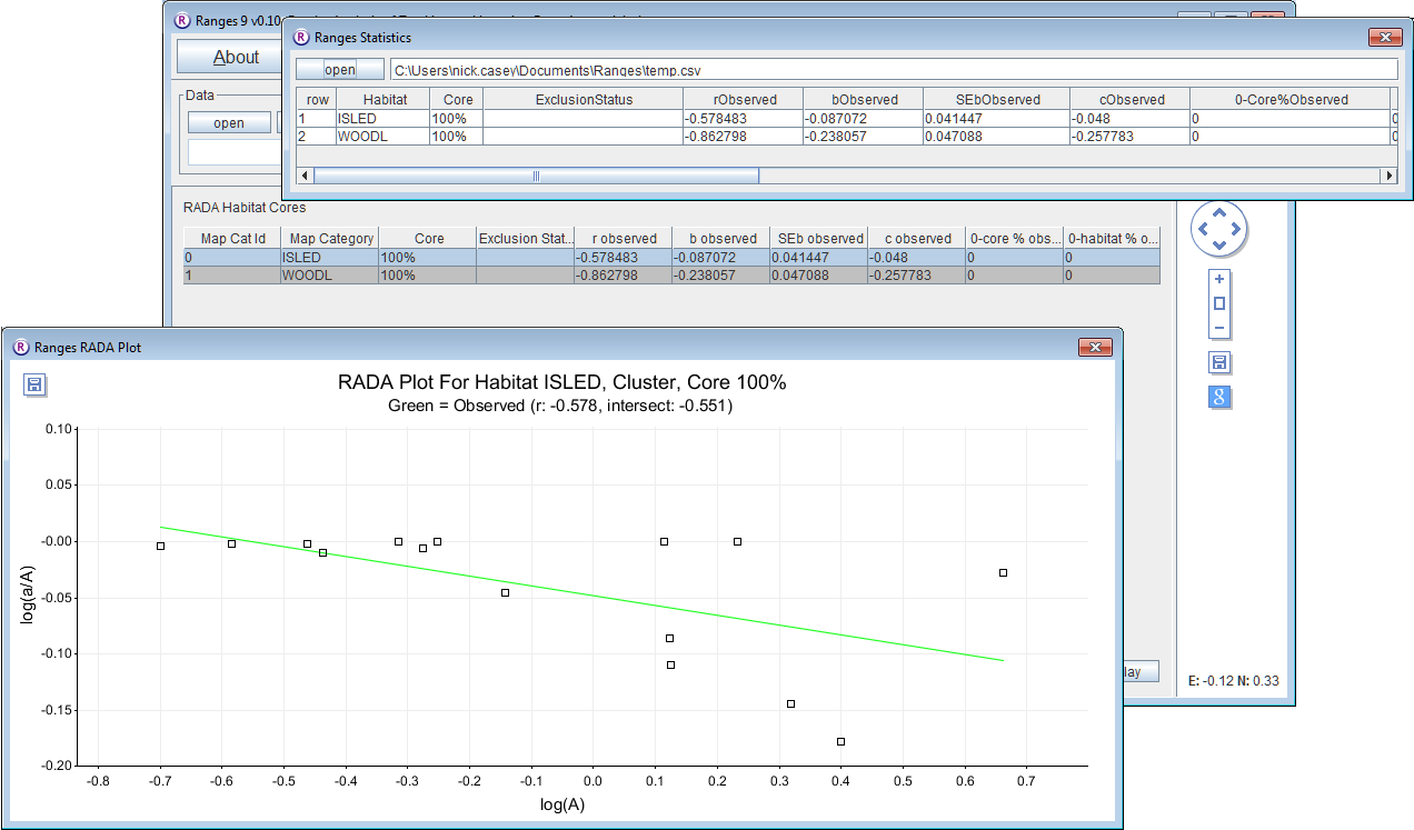
- Click on the Modelling button to open the setup window.
- Select resource area dependence.
- Under Map file press browse and find the file <RangesFolder>\samples\squirrel\furhab.ves.
- Similarly, under Edge file press browse and find the file <RangesFolder>\samples\squirrel\furzey_cxoi01s.edg.
If that file is not in the folder, you need to create it in the Tutorial sequence Cluster analysis with objective cores.
- Under Analysis Options select observed only
- Press the Run Analysis button.
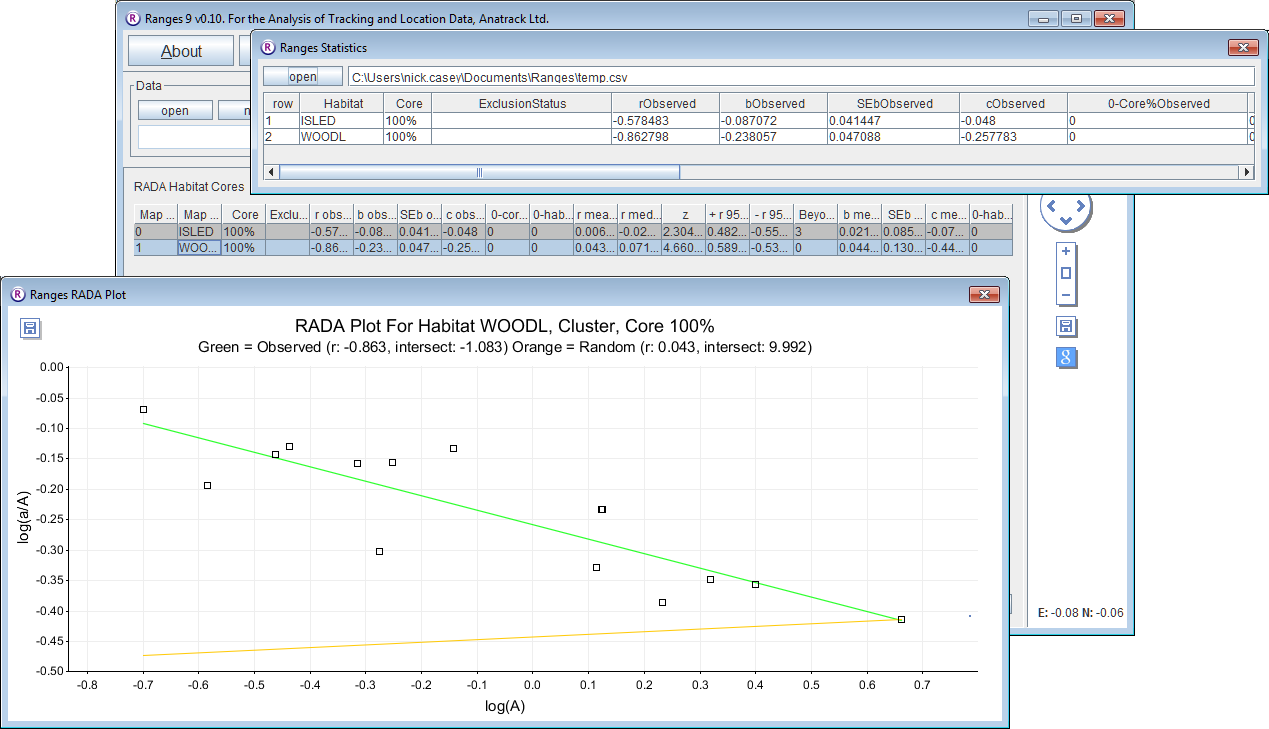
The computer does 15 habitat analyses and displays the results in a graph of the log proportion of resource on the log area of the range. As the first resource is the area of island inclusive of woodland (and thus unlike the exclusive habitat areas in most habitat analysis), it fills the range of most of the 15 squirrels, but six of them also included appreciable proportions of oil-extraction area which is not included as usable island; as these squirrels also had the larger range outlines there is a negative correlation (r = -0.579), which repeats in the statistics window. If you click WOODL at the top left of the main window, the graph shows a stronger relationship (r = -0.863) with steeper green regression line. The prediction of minimum woodland area required, from the intercept c, is 10^-1 and therefore about 0.1 ha.
Comparing observed and random data
- Click on the Modelling button to open the setup window.
All the previous options and files should still be selected, but make them again if not
- Under Analysis Options select observed and 199 random iterations
- Press the Run Analysis button.
- Have a cup of tea or coffee while your computer does more than 3,000 habitat analyses.
This time the graph includes a yellow line based on the mean slope b and intercept c for the regressions from 199 random samplings with replacement among the 15 observed range outlines, each of which was randomly rotated and displaced within the envelope round all the observed outlines in a separate window; these mean values are given in the statistics window, also with 95% confidence limits for r assuming a normal distribution, and a z value for the difference between the observed r and that mean value. However, the most robust statistic for tests is in the next column: the number of negative random values beyond the observed r. The value will vary with each run, but will average about 3. In a two-tailed test with 200 samples (including the observed), P < 0.05 for a value less than 5. For WOODLand, there are no random values beyond the observed (i.e. P < 0.01), nor in repeated runs with 999 iterations (i.e. P < 0.002).
- Now under envelope select user defined, after making a file with an expansive outline (e.g. 99% ellipses)
You will find with this particular file that, due to the greater availability of sea round the island for random outlines, nearly 10% of the random outlines are in the sea if using either the default replace zeros or the option ignore zeros. In these circumstances the random regressions have a tendency to be positive, because small range outlines have a greater chance of including no island or woodland. The option resample zeros is then most conservative, because it forces random samples to contain habitat and tends to produce regression with b=0.
Kaplan Meier Survival Analysis
Plotting survival for a single data set

- Click on the Modelling button to open the setup window.
- Select kaplan meier survival.
- Under Analysis Options ensure one set is selected
- Under Input files press browse and find, for the set 1 survival file the file <RangesFolder>\samples\goshawk\Juv_Male.srv.
- Press the Run Analysis button.
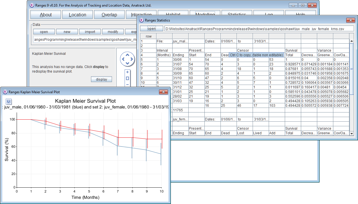
Looking at the statistics window, the sample size was not adequate until the start of the second month, and became less than 30 animals due to moulting of tail-mounted radio tags after 30 April. Run the analysis again, selecting as set 1 start date the specified date and use the calendar to select 1 July 1980 (around the fledging date), then in set 1 end date again select specified date and set 31 March 1981. This estimates juvenile male survival to the start of the next egg-laying period, as used in Kenward et al. (1999).
Comparing two sets of survival data
- Under Analysis Options select two sets for comparison
- Under Input files check that the set 1 survival file is still <RangesFolder>\samples\goshawk\Juv_Male.srv.
- Check that set 1 start date has specified date selected, of 1 July 1980.
- Check that set 1 end date has specified date selected, of 31 March 1981.
- Press browse for the set 2 survival file and find <RangesFolder>\samples\goshawk\Juv_Female.srv.
- For the set 2 start date, use the set 1 start date option.
- For the set 2 end date, use the set 2 end date option.
- Press the Run Analysis button.
The survival is poorer for juvenile males than for juvenile females due mainly to differences from October (month 4) onwards. The z values of 2.07 to 2.13 are higher than the value of 1.96 for alpha = 0.05, so P < 0.05.
Data Sources
The squirrel data were collected in the 1980s, before the introduction of location qualifying variables: the data therefore consist of simple x,y coordinates. One set, which was collected at Elton Estate in work conducted from Monks Wood Experimental Station, was used to illustrate the introduction of compositional analysis (Aebischer et al. 1993). A second set, collected on Furzey Island in Poole Harbour in work conducted from Furzebrook Research Station, was used to illustrate the effectiveness of Cluster analysis in Kenward (2001), Kenward et al. (2001).
The buzzard data were collected for a study of relationships between demography and habitat conducted from Furzebrook Research Station (Kenward et al. 2000, 2001, South & Kenward 2001, Walls & Kenward 1995, 1998, 2001). Note that some of the buzzard data have been altered slightly to avoid use used without the authors' permission. Goshawk survival data were collected on the Swedish island of Gotland (Kenward et al. 1993, 1999); the natal year of all fledged cohorts has been set to 1980 in the example files.
The blackbird data represent material on an abundant European passerine species collected by Ben Kenward during a pilot study for work on garden birds. There are two adult males, an adult female that was incubating eggs and one that was not breeding at the time. All but the breeding female foraged in a garden during the day and roosted at night in a Rhododendron thicket some 200m away across an open field. The birds were tracked on foot, and locations for triangulation taken from less than 100m away, giving a tracking resolution of about 10m. For this reason, coordinates were entered in 10m units.
The lion data come from 3 lions (2 females and 1 male), GPS collared in Botswana by Graham Hemson of the Wildlife Conservation Research Unit, Oxford (see Hemson et al. 2005). The collars were scheduled to take 15 locations in every 24 hour period and the sample given here is for October 2001. The data coordinates are expressed in the UTM projection. In the first half of the month the movements of the first female are restricted to an area approximately 10 x 10 km in the west. Then over the following 10 days she makes a return trip of over 70 km coinciding with the start of the zebra and wildebeest migrations. The movements of the 2nd female and the male are very similar at the start of the month. Later in the month the male makes an excursion into an area crossed by the first female about a week beforehand.
The squirrel, buzzard and goshawk data came from work funded by the UK Natural Environment Research Council in its Centre for Ecology and Hydrology (formerly Institute of Terrestrial Ecology), in the last case in cooperation with Uppsala University and the Swedish Hunters' Association. The blackbird and lion data were collected during student and post-graduate projects from the University of Oxford, the first supervised externally within NERC-CEH. The files within the folder fish are a simulated dataset created by Sean Walls.