Interaction Analysis
Introduction
The general purpose of these routines is to analyse spatial interactions between animals or between patterns of locations (spatial and temporal) for individual animals. Autocorrelation analyses spatio-temporal relationships between locations, which can help to identify optimal sampling intervals for recording home ranges from data collected in a pilot study. Analysis of dynamic interactions is a complement to the static interactions that are described by the overlap analysis of home range outlines, because it examines whether animals tended to cohere or avoid each other within home ranges that overlapped strongly (for example because the animals were sibs or clan-mates). Investigation of whether location-point distances differ from random spacing can reveal whether animals favoured or avoided particular points, for example the dens of other individuals. Examination of range centre spacing can reveal whether animals tended to distribute themselves at random, or in regular patterns that suggest avoidance, or in clumps that suggest cohesion.
Autocorrelations
Autocorrelation analysis examines the way that distances between locations change with sampling intervals. It is, therefore, useful for estimating the optimal time interval to use between recording consecutive locations. If locations are recorded with short time intervals, individuals will not have had time to travel far. As a result there will be high spatio-temporal dependence between locations, and more locations will be required to define a home range (Harris et al. 1990). The originators of the technique (Swihart & Slade 1985) suggested that locations could be considered spatio-temporally independent if they met a randomness criterion by having 3 consecutive values of Schoener’s index scoring greater than 2. This estimated a "time to independence" for recording intervals. However, the estimation is based on a circular normal distribution of locations. This is often unrealistic, because animals create multimodal (multinuclear) ranges by favouring particular areas for food, nests and travel - in other words their locations are never truly independent and should not be treated as such in analyses (Kenward 1992, Otis & White 1999).
Swihart & Slade (1987) showed that their "time to independence" had value for investigating home range activity, because it estimates a measure of time to cross a home range. However, animals often move in ways that fail to meet the independence criteria for several days, if at all, such that taking locations at intervals greater than the "time to independence" under-samples their home range. A general value of Schoener’s index for a sampling interval at which the least number of locations define a home range has yet to be determined, but may lie closer to 1 than to 2 (Kenward 2001).
As time intervals are integral to the analysis, suitable location files must include correctly labelled time location-qualifying variables. Following the format used by the originators of the technique (Swihart & Slade 1985), the programme plots increasing sampling intervals in minutes on the x-axis and Schoener's index on the y-axis.
Schoener's index indicates the degree of independence between distance and time. If the value of the index is low, this indicates a high correlation between distance and time, e.g., because during short sampling intervals the animal did not have time to move far before it was next located.
The programme works through the sequence of locations from start to finish for each set of sampling intervals. It then tests for correlations between distance and time for this set. If using a 5-minute minimum interval the routine first estimates distances for all locations from 2.5 to 7.5 minutes apart and estimates the Schoener (1981) index V (= mean squared distances between locations / mean squared distance from each location to the arithmetic activity centre). It then processes those between 7.5 to 12.5 minutes apart and so on up to the default maximum of 48 hours apart.
Minimum time intervals
This allows you to alter the length of the sample interval. This is by default based on the minimum time interval within your data file. Choosing an appropriate interval is important. If, for example, locations have been taken approximately one hour apart, there may be too few locations to estimate in Schoener's index using 5 minute sampling intervals (i.e., 57.5 to 62.5, 62,5 to 67.5 etc.). However, good results may be obtained with 30-minute sampling intervals (i.e., 45 to 75 etc.). However, note that there may also tend to be few records of very long time intervals, so that plots often start smoothly and then become "ragged" as variance of the index increases with reduction in sample size.
Plot time
This allows you to set the total length of time of the recording period to be used in the analysis. The default is to plot the estimate for 48 hours. Be careful to pick an appropriate time scale for the data that you have. It is very easy not to.
Results plots
These are displayed in the chart window for each range. Selecting different Ranges within the ranges table will display the corresponding autocorrelation plot and locations. A green line shows where a Schoeners index of 1 is exceeded by 3 consecutive locations, and an orange line where a Schoeners index of 2 is exceeded by 3 consecutive locations. The time where a Schoeners value of 2 is exceeded is put into the output file as TTISchoeners2(hours) – this is the "Time To Independence" estimator proposed by Swihart & Slade 1985. The output file is automatically loaded into the Statistics window.
Dynamic interactions
This analysis routine gives a single "cohesion" index, for the tendency of pairs of animals to be close together at the same time. Animals shown to share large areas in overlap analyses may seldom encounter each other because they rarely visit the same place at the same time. Macdonald et al (1980) called the analysis of overlapping range outlines "static interaction" and they proposed the examination of "dynamic interaction" by looking at locations taken at the same time. The original publication provided a test of whether 2 individuals showed significant attraction or avoidance, but this depended on two assumptions. Firstly, that locations are statistically independent and secondly, that their distribution fitted a parametric model. Ranges avoids assumptions about independence and distributions of locations between single pairs of individuals.
The programme provides a single statistic for each range as described in Kenward et al (1993). The observed and possible distances between animals are compared. The mean, geometric mean and median distances are estimated between the n observed pairs of same-time locations for animal 1 and 2. Then the equivalent values are estimated for the n x n possible distances if animal 2 could be at any of its n used positions when animal 1 was at each of its used positions. The observed and possible distances are compared using Jacob's Index (Jacobs 1974). This gives a value of 0 if the observed and possible distances were the same, rising towards +1 if observed distances were small relative to possible distances (because the animals were usually together) or falling towards -1 if animals tended to avoid each other. This gives a single index for each pair of animals, which tends to be most consistent if based on the geometric mean distances (Walls & Kenward 2001).
Individual selection
all
Use this if all the animals share overlapping ranges, for example through being a single family.
overlapping quadrats
This uses a rectangular edge around the W E S and N limits of ranges to select animals which have overlapping quadrats for estimation of range overlaps.
overlapping ranges
This examines animals with ranges which overlap, and requires the input of a range overlap matrix created in overlap analysis.
the same focal site
If many families are combined in a file, you can use this to confine the analysis to those at the same den or other focal site.
Same time observations defined by
sequence of locations
This is appropriate if there are equal numbers of locations for each animal, recorded at roughly the same time on each occasion (i.e. by repeated sampling round all the tagged animals). The analysis will still work if a few animal locations were scored as missing (-9,-9). The missing values merely reduce n for all pairs involving that animal.
time attributes of locations
For this to work the location file must contain correctly labelled location-qualifying variables which define the times that locations were recorded. You will need to input a ‘threshold between same time observations’, to make allowance for records that were actually recorded 5 minutes apart but can be considered simultaneous. Locations further apart than this threshold will be treated as missing and excluded from the analysis.
Maximum randomisation sample
The set of all possible pairs of locations is n x n, where n is the maximum locations recorded for any individual. This number can become very large for large sample sizes, which makes the analyses slow, due to the ranking process that determines median values, and also require excessive memory. In this case, very little extra variation will result if the total is boot-strapped, to select at random a smaller sample within the set n x n. This is useful to make analyses of large datasets run faster. Selection of a sample from n x n occurs automatically to limit sample size if n x n is greater than 5000. The user-interface will accept values between 500 & n x n.
Location-point distances
This option allows you to estimate whether an animal has been tending to approach or avoid sites associated with other animals, such as nests or scent marks. To use it, you require a location file and a site file. The latter can either be a file of locations or of habitat points. Habitat shape files may be used to refine the analysis by defining envelopes for random sampling operations.
The routine starts by producing a single sample of nearest-site distances for a set of random locations within a defined envelope. It then estimates the observed distances of each location from the nearest site for each set of locations. The observed distances are then compared to the expected distances (from the random locations) in a process very similar to that used for dynamic interactions to give a Jacobs' Index of avoidance or cohesion. The arithmetic mean, geometric mean and median distances are also displayed (or exported in a statistics file) so that the size of the difference can be seen.
It is important to note that the results of the analysis are boundary-dependent. Imagine setting an extensive envelope for random locations, far beyond the area used by animals. The animal locations would then tend always to be closer than random locations to the point-sites. On the other hand, setting a envelope smaller than the size of home ranges may create an opposite effect. It is therefore not really possible to test for absolute cohesion or avoidance in this analysis, but it is useful for comparing different categories of animal or times of year if the same analysis criteria are used throughout. For further explanation and use of this analysis, see Walls & Kenward (2001).
Envelope
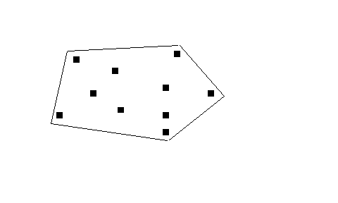
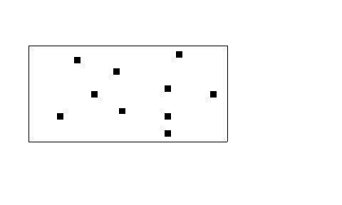
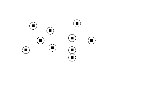
The envelope within which random locations are thrown, and within which observed locations are used, can either be a polygon around all the points (Inclusive or User-defined), or a circle around each point (Point-centred circle).
inclusive polygon
This places a envelope around the outside to include all the points. In this case a point file will have been entered, either as a location file or habitat point file. Then you will be asked to choose the buffer strip, which is the distance outside all the locations that the polygon is drawn. This should be relevant to the distribution of the points and therefore it is based on the nearest neighbour distances (please see below).
user-defined envelope
The envelope can be defined by a vector shape or an edge file, for example to delimit the study area create a vector shape file containing the corners of the study area.
point-centred circles
This analysis is really useful for isolated points between which there are areas that the animals are unlikely to use. If random locations are thrown into areas that the animals themselves are unlikely to use it will obviously produce an unwanted bias to the expected distances.
The size of the buffer strip in the last two methods is based on the nearest-neighbour distances of the points, so that it is biologically meaningful.
Buffers
The choice here depends on whether you are testing for attraction to sites, or avoidance of sites. When testing for attraction, the conservative approach is to use a narrow buffer to create a small envelope around sites, perhaps using the minimum nearest neighbour distance or the very conservative boundary suppression of the final option. When testing for avoidance, the conservative approach is to use a large buffer, the maximum nearest neighbour distance, to create a large envelope. Using the mean nearest-neighbour distance may be slightly biased in either direction, but is useful for an initial run, to check whether significant attraction or avoidance is likely.
mean n-n distance / 2
Half of the mean nearest-neighbour distance.
max n-n distance / 2
Half of the maximum nearest-neighbour distance.
min n-n distance / 2
Half of the minimum nearest-neighbour distance.
suppressed
No buffers.
Maximum randomisation sample
Select the size of the "randomisation sample" (the number of random locations used in the analysis). Small random samples increase the speed of runs (e.g. for a preliminary assessment), whereas large random samples minimise the sampling variation in the results. The minimum sample permitted is 500.
Range centre spacing
The final interaction analysis provides tests for spacing of range centres, using conventional nearest neighbour analysis (Clarke & Evans 1954). The minimum input required is a range-edge file containing a single core of convex polygons, ellipses or contours (concave polygons and cluster analysis outlines lack centres). Go to location analyses for details on creating these polygon files. The results indicate whether centres are more regularly spaced both than an expected normal distribution, and also than spacing based (by default) on 1000 random locations. In each case, as in the original publication, Student's t is used to test for significantly regular spacing. These results are displayed on the final screen and can be filed.
When using random points, note that the results of the analysis could be envelope-dependent, especially if the distribution is being estimated within an irregular envelope. Setting an extensive envelope for random locations means that higher regularity will occur in the random sample than when an area is, say, long and narrow.
The way in which buffers define envelopes can be seen above.


